
[인공지능] TensorFlow train_test_split
- 인공지능
- 2023. 3. 5. 15:40

소개
- 앞서 TensorFlow 학습 예제코드는 numpy 에서 직접 데이터를 손으로 잘라서 사용했습니다.
- 하지만, 사이킷 런에서는 이미 잘 구현된 train_test_split 함수를 제공해 주고 있습니다.
train_test_split 함수 사용 법
from sklearn.model_selection import train_test_split
x_train, x_test, y_train, y_test = train_test_split(
  x, y, random_state=66, test_size=0.4, shuffle = False
)- x, y에 데이터의 x값과 y값을 넣습니다.
- text_size=0.4 는 test_size가 40% 라는 의미입니다.
- 마찬가지로 train_size=0.6 이라고도 할 수 있습니다.
- 즉, train이 60%, test 가 40% 로써 동일한 결과가 됩니다.
- shuffle 은 데이터를 섞어주는 역할을 합니다.
- True 인 경우 데이터를 섞게 되고, False인 경우 섞지 않습니다.
- 예를 들어, X=(1,2,3), y=(4,5,6) 일 경우 데이터를 shuffle 한다고 해서 X=(2,3,1), y=(4,6,5) 이런식으로 x와 y의 순서까지는 바뀌지 않습니다.
- 1과 4,2 와 5,3 과 6 의 쌍 자체가 바뀌지는 않습니다.
- shuffle이 true 인 경우 x=(2,3,1) 로 섞이게 되면 y=(5,6,4) 가 됩니다.
train_test_split 함수 예제 코드
- 그럼 실제 train_test_split 함수 예제 코드를 작성하여 학습을 진행해 보도록 하겠습니다.
import numpy as np
import matplotlib.pyplot as plt

from tensorflow import keras
from sklearn.model_selection import train_test_split


#1 데이터
x = np.array(range(1, 101))
y = np.array(range(1, 101))

x_train, x_test, y_train, y_test = train_test_split(
    x, y, random_state=66, test_size=0.4, shuffle=False
)

# test 데이터의 50%를 배분하여
# train:val:test의 비율이 6:2:2 가 됨
x_val, x_test, y_val, y_test = train_test_split(
    x_test, y_test, random_state=66, test_size=0.5
)

# Keras의 Sequential모델을 선언
model = keras.Sequential([
    # 첫 번째 Layer: 데이터를 신경망에 집어넣기
    keras.layers.Dense(32, activation='relu', input_shape = (1, )),
    # 두번째 층
    keras.layers.Dense(32, activation='relu'),
    # 세번째 출력층: 예측 값 출력하기
    keras.layers.Dense(1)
])

# 모델을 학습시킬 최적화 방법, loss 계산 방법, 평가 방법 설정
model.compile(optimizer='adam',loss='mse',metrics=['mse', 'binary_crossentropy'])

# 모델 학습
history = model.fit(x_train, y_train, epochs = 1000, batch_size = 1,
                    validation_data=(x_val, y_val))

# 평가 예측
mse = model.evaluate(x_test, y_test, batch_size=1)
print(f"mse : {mse}")

y_predict = model.predict(x_test)
print(y_test)

# 결과를 그래프로 시각화
plt.scatter(x_test, y_test, label='y_true')
plt.scatter(x_test, model.predict(x_test), label='y_pred')
plt.legend()
plt.show()
실행 결과
- 실행 결과 정상적으로 학습되어 Predict 값이 실제 값이랑 매우 비슷한 것을 확인할 수 있습니다.
mse : [1.146524755313294e-05, 1.146524755313294e-05, -1216.1268310546875]
[ 65  80  91  66  62  96  64  89  92 100  93  86  85  78  70  75  69  73
  84  97]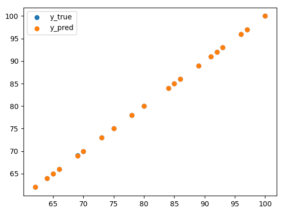
728x90
'인공지능' 카테고리의 다른 글
| [인공지능] TensorFlow 2.x과 1.x의 차이점 (0) | 2023.03.04 |
|---|---|
| [인공지능] Keras 모델 (0) | 2023.03.03 |
| [인공지능] Keras 모델 생성 기본 구조 (0) | 2023.03.03 |
| [인공지능] TensorFlow 데이터 분리 (0) | 2023.02.26 |
| [인공지능] MNIST 모델별 Image Resize 하기 (0) | 2023.02.26 |


