
[인공지능] TensorFlow 회귀 분석 모델
- 인공지능
- 2022. 2. 15. 16:55

참조
선형 회귀(Linear Regression)
from cProfile import label
import numpy as np
import tensorflow as tf
import matplotlib.pyplot as plt

plt.style.use('seaborn-white')

learning_rate = 0.01
training_steps = 1000

X = np.random.randn(50) # 입력 값
Y = 2*X + np.random.randn(50) # 실제 값

W = tf.Variable(np.random.randn(), name='weight')
b = tf.Variable(np.random.randn(), name='bias')

def linear_regression(x):
    return W * x + b

# 손실 함수(loss)
def mean_square(y_pred, y_true):
    return tf.reduce_mean(tf.square(y_pred - y_true))

optimizer = tf.optimizers.SGD(learning_rate)

def run_optimization():
    with tf.GradientTape() as tape:
        pred = linear_regression(X)
        loss = mean_square(pred, Y)

    gradients = tape.gradient(loss, [W, b])

    optimizer.apply_gradients(zip(gradients, [W, b]))

for step in range(1, training_steps + 1):
    run_optimization()

    if step % 50 == 0:
        pred = linear_regression(X)
        loss = mean_square(pred, Y)
        print("step : {:4d}\tloss:{:.4f}\tW: {:.4f}\tb:{:.4f}".format(step, loss, W.numpy(), b.numpy()))

plt.plot(X, Y, 'ro', label='Data')
plt.plot(X, np.array(W * X + b), label='Fitted Line')
plt.legend()
plt.grid()
plt.show()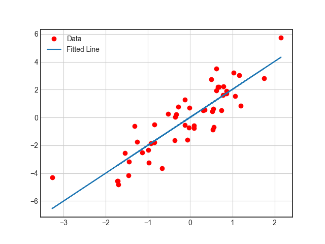
다항 회귀(Nonlinear Regression)
import numpy as np
import tensorflow as tf
import matplotlib.pyplot as plt
from tensorflow.keras.optimizers import Adam
epochs = 1000
learning_rate = 0.04
a = tf.Variable(np.random.randn())
b = tf.Variable(np.random.randn())
c = tf.Variable(np.random.randn())
print(a.numpy())
print(b.numpy())
print(c.numpy())
# 데이터 지정
X = np.random.randn(50)
Y = X**2 + X*np.random.randn(50)
line_x = np.arange(min(X), max(X), 0.001)
line_y = a*line_x**2 + b*line_x + c
x_ = np.arange(-4.0, 4.0, 0.001)
y_ = a*x_**2 + b*x_+c
plt.scatter(X, Y, label='X data')
plt.plot(x_, y_, 'g--', label='origin line')
plt.plot(line_x, line_y, 'r--', label='before train')
plt.xlim(-4.0, 4.0)
plt.legend()
plt.grid()
plt.show()
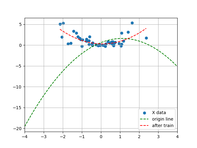
# Util Functions
def compute_loss():
pred_y = a*(np.array(X)**2) + b*np.array(X) + c
loss = tf.reduce_mean((Y - pred_y)**2)
return loss
# Optimizer
optimizer = Adam(learning_rate=learning_rate)
# 학습
for epoch in range(1, epochs + 1, 1):
optimizer.minimize(compute_loss, var_list=[a,b,c])
if epoch % 100 == 0:
print("epoch: {:4d}\ta: {:.4f}\tb: {:.4f}\tc:{:.4f}".format(epoch, a.numpy(), b.numpy(), c.numpy()))
line_x = np.arange(min(X), max(X), 0.001)
line_y = a*line_x**2 + b*line_x + c
plt.scatter(X, Y, label='X data')
plt.plot(x_, y_, 'g--', label='origin line')
plt.plot(line_x, line_y, 'r--', label='after train')
plt.xlim(-4.0, 4.0)
plt.legend()
plt.grid()
plt.show()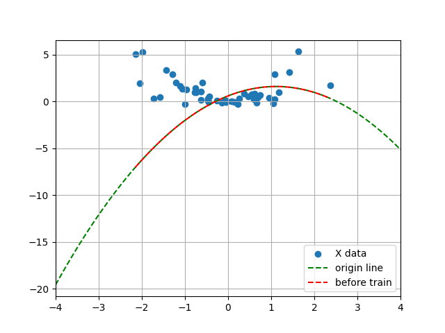
로지스틱 회귀(Logistic Regression)
- 다항 분류, MNIST
import numpy as np
import tensorflow as tf
import matplotlib.pyplot as plt
from tensorflow.keras.datasets import mnist

# 하이퍼 파라미터
num_classes = 10
num_features = 784

learning_rate = 0.1
training_steps = 1000
batch_size = 256

# 데이터 로드
(x_train, y_train), (x_test, y_test) = mnist.load_data()

x_train, x_test = np.array(x_train, np.float32), np.array(x_test, np.float32)

x_train, x_test = x_train.reshape([-1, num_features]), x_test.reshape([-1, num_features])

x_train, x_test = x_train / 255., x_test / 255.

# tf.data API 사용
train_data = tf.data.Dataset.from_tensor_slices((x_train, y_train))
train_data = train_data.repeat().shuffle(5000).batch(batch_size).prefetch(1)

# 변수 지정
W = tf.Variable(tf.random.normal([num_features, num_classes]), name='weight')
b = tf.Variable(tf.zeros([num_classes]), name='bias')

# Util Functions
def logistic_regression(x):
    return tf.nn.softmax(tf.matmul(x, W) + b)

def cross_entropy(pred_y, true_y):
    true_y = tf.one_hot(true_y, depth=num_classes)
    pred_y = tf.clip_by_value(pred_y, 1e-9, 1.)

    return tf.reduce_mean(-tf.reduce_sum(true_y * tf.math.log(pred_y), 1))

def accuracy(y_pred, y_true):
    correct_prediction = tf.equal(tf.argmax(y_pred, 1), tf.cast(y_true, tf.int64))
    return tf.reduce_mean(tf.cast(correct_prediction, tf.float32))

# Optimizer
optimizer = tf.optimizers.SGD(learning_rate)

def run_optimization(x, y):
    with tf.GradientTape() as tape:
        pred = logistic_regression(x)
        loss = cross_entropy(pred, y)

    gradients = tape.gradient(loss, [W, b])

    optimizer.apply_gradients(zip(gradients, [W, b]))

# 학습 진행
for step, (batch_x, batch_y) in enumerate(train_data.take(training_steps), 1):
    run_optimization(batch_x, batch_y)

    if step % 50 == 0:
        pred = logistic_regression(batch_x)
        loss = cross_entropy(pred, batch_y)
        acc = accuracy(pred, batch_y)
        print("step: {:4d}\tloss: {:.4f}\taccuracy: {:4f}".format(step, loss, acc))

# 테스트
pred = logistic_regression(x_test)
print("Test Accuracy : {}".format(accuracy(pred, y_test)))

# 시각화
num_images = 5
test_images = x_test[:num_images]
predictions = logistic_regression(test_images)

plt.figure(figsize=(14, 8))

for i in range(1, num_images + 1, 1):
    plt.subplot(1, num_images, i)
    plt.imshow(np.reshape(test_images[i-1], [28, 28]), cmap='gray')
    plt.title("Model prediction: {}".format(np.argmax(predictions.numpy()[i-1])))

plt.show()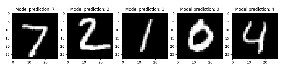
728x90
'인공지능' 카테고리의 다른 글
| [인공지능] 케라스 기초 - 주요 레이어 (0) | 2022.02.15 |
|---|---|
| [인공지능] 케라스 기초 - 주요 레이어 import 하는 방법 (0) | 2022.02.15 |
| [인공지능] TensorFlow 간단한 신경망 구조 (0) | 2022.02.14 |
| [인공지능] TensorFlow 기초 문법 (0) | 2022.02.14 |
| [인공지능] TensorFlow GPU 동작 확인 방법 (0) | 2022.02.10 |


