
[인공지능] TensorFlow 데이터 분리
- 인공지능
- 2023. 2. 26. 09:33

목적
- 앞서 TensorFlow Validation 코드에서는 데이터를 분리하지 않고 일일이 사용했습니다.
- 이번에는 데이터를 일일이 쓰지 않고, 좀 더 많은 데이터를 잘라서 사용해 보도록 하겠습니다.
- 예제는 1부터 100까지의 데이터를 준비 했습니다.
예제 코드
- 6:2:2 비율로 Train, Valid, Test 데이터 셋을 분리한 예제 코드입니다.
import numpy as np
import matplotlib.pyplot as plt

from tensorflow import keras


#1 데이터
x = np.array(range(1, 101))
y = np.array(range(1, 101))

# 6:2:2 비율로 Train:Valid:Test 셋 나눔
x_train = x[:60]
x_val = x[60:80]
x_test = x[80:]

y_train = y[:60]
y_val = y[60:80]
y_test = y[80:]

# Keras의 Sequential모델을 선언
model = keras.Sequential([
    # 첫 번째 Layer: 데이터를 신경망에 집어넣기
    keras.layers.Dense(32, activation='relu', input_shape = (1, )),
    # 두번째 층
    keras.layers.Dense(32, activation='relu'),
    # 세번째 출력층: 예측 값 출력하기
    keras.layers.Dense(1)
])

# 모델을 학습시킬 최적화 방법, loss 계산 방법, 평가 방법 설정
model.compile(optimizer='adam',loss='mse',metrics=['mse', 'binary_crossentropy'])

# 모델 학습
history = model.fit(x_train, y_train, epochs = 1000, batch_size = 1,
                    validation_data=(x_val, y_val))

# 평가 예측
mse = model.evaluate(x_test, y_test, batch_size=1)
print(f"mse : {mse}")

y_predict = model.predict(x_test)
print(y_test)

# 결과를 그래프로 시각화
plt.scatter(x_test, y_test, label='y_true')
plt.scatter(x_test, model.predict(x_test), label='y_pred')
plt.legend()
plt.show()
실행 결과
- 학습 결과, mse 값도 대체적으로 낮으면서 예측값과 실제값이 거의 정확하게 일치하는 것을 확인할 수 있습니다.
mse : [2.318470251339022e-05, 2.318470251339022e-05, -1364.806884765625]
[ 81  82  83  84  85  86  87  88  89  90  91  92  93  94  95  96  97  98
  99 100]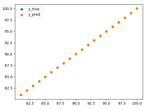
테스트 데이터 변경
- 위에서는 x_test 값으로 Predict 진행하였습니다.
- 하지만 가급적이면 test 한 값 보다는 새로운 데이터로 예측하는 것이 더 좋다고 합니다.
- 때문에 x_predict 를 새로 입력하여 값을 다시 예측해 보도록 코드를 아래와 같이 변경하였습니다.
import numpy as np
import matplotlib.pyplot as plt

from tensorflow import keras


#1 데이터
x = np.array(range(1, 101))
y = np.array(range(1, 101))

# 6:2:2 비율로 Train:Valid:Test 셋 나눔
x_train = x[:60]
x_val = x[60:80]
x_test = x[80:]

y_train = y[:60]
y_val = y[60:80]
y_test = y[80:]

# Keras의 Sequential모델을 선언
model = keras.Sequential([
    # 첫 번째 Layer: 데이터를 신경망에 집어넣기
    keras.layers.Dense(32, activation='relu', input_shape = (1, )),
    # 두번째 층
    keras.layers.Dense(32, activation='relu'),
    # 세번째 출력층: 예측 값 출력하기
    keras.layers.Dense(1)
])

# 모델을 학습시킬 최적화 방법, loss 계산 방법, 평가 방법 설정
model.compile(optimizer='adam',loss='mse',metrics=['mse', 'binary_crossentropy'])

# 모델 학습
history = model.fit(x_train, y_train, epochs = 1000, batch_size = 1,
                    validation_data=(x_val, y_val))

# 평가 예측
mse = model.evaluate(x_test, y_test, batch_size=1)
print(f"mse : {mse}")

x_predict = np.array(range(101, 111))

y_predict = model.predict(x_predict)
print(y_predict)

# 결과를 그래프로 시각화
plt.scatter(x_predict, y_predict, label='y_true')
plt.scatter(x_predict, model.predict(x_predict), label='y_pred')
plt.legend()
plt.show()
실행 결과
- 101 부터 110 까지 값이 정확하게 얘측 된 것을 확인할 수 있습니다.
mse : [5.7480065152049065e-09, 5.7480065152049065e-09, -1364.806884765625]
[[100.999916]
 [101.999916]
 [102.9999  ]
 [103.9999  ]
 [104.9999  ]
 [105.99989 ]
 [106.9999  ]
 [107.9999  ]
 [108.999886]
 [109.999886]]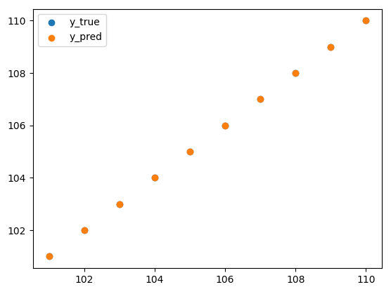
728x90
'인공지능' 카테고리의 다른 글
| [인공지능] Keras 모델 (0) | 2023.03.03 |
|---|---|
| [인공지능] Keras 모델 생성 기본 구조 (0) | 2023.03.03 |
| [인공지능] MNIST 모델별 Image Resize 하기 (0) | 2023.02.26 |
| [인공지능] Tensorflow Validation 추가 (0) | 2023.02.25 |
| [인공지능] Tensorflow 1에서 100까지 값 예측하기 (0) | 2023.02.24 |


